Well, we all know every algorithm has it’s own merits and shortcomings. So, comparing them head-on is not a logical thing to do. It depends on the type of data, type of analysis we are performing and the dataset itself. In this post, I’m going to use the famous/infamous wine dataset to perform supervised machine learning and compare these algorithm:
- LinearRegression
- RandomForestRegressor
- GradientBoostingRegressor
- SVR
- KNeighborsRegressor
Ok, let’s get on with our business.
1. Importing Essentials
# Pandas and numpy for data manipulation
import pandas as pd
import numpy as np

# No warnings about setting value on copy of slice
pd.options.mode.chained_assignment = None

# Display up to 60 columns of a dataframe
pd.set_option('display.max_columns', 60)

# Matplotlib visualization
import matplotlib.pyplot as plt
%matplotlib inline

# Set default font size
plt.rcParams['font.size'] = 24

# Internal ipython tool for setting figure size
from IPython.core.pylabtools import figsize

# Seaborn for visualization
import seaborn as sns
sns.set(font_scale = 2)

# Splitting data into training and testing
from sklearn.model_selection import train_test_split
plt.style.use('classic')
from sklearn.preprocessing import Imputer, MinMaxScaler

from sklearn.linear_model import LinearRegression
from sklearn.ensemble import RandomForestRegressor, GradientBoostingRegressor
from sklearn.svm import SVR
from sklearn.neighbors import KNeighborsRegressor

# Hyperparameter tuning
from sklearn.model_selection import RandomizedSearchCV, GridSearchCV
2. Reading data
# Read in data into a dataframe
data = pd.read_csv('wine.data')

# Display top of dataframe
data.info()
3. Figuring out dependencies of features
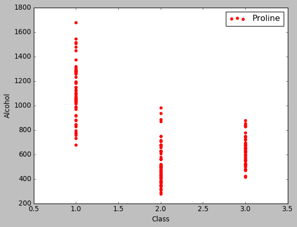
The next step should be to see how and if each feature affects our target (class in our case). One way to do this is by using seaborn and plotting multiple relationships with facets. As the wine dataset is very common, for demonstrtion puposes, i will just plot the target’s relationship with Alcohol:
plt.style.use('classic')
plt.scatter(data.Class,data.Proline,marker = 'o',label = 'Proline',color = 'red')
plt.xlabel('Class'); plt.ylabel('Alcohol')
plt.legend();
4. Dividing into training and validation datasets
Now, we will divide our dataset into training and test datasets. For this, we must remove the target from the main set and place it in another.
features = data.drop(columns = 'Class')
targets = pd.DataFrame(data['Class'])
X, X_test, y, y_test = train_test_split(features, targets, test_size = 0.3, random_state = 42)
5. Scaling features
Every feature has different values; for example Alcohol ranges from ~200 to ~700 and Color intensity has a range from 1.28 to 13. When we feed these features into our model, Alcohol will clearly have more precedence over Color intensity. To avoid this, we need to scale our features. This can be done easily by using scikit-learn’s MinMaxScaler. Here i will scale my features from 0 to 1:
scaler = MinMaxScaler(feature_range=(0, 1))
scaler.fit(X)
X = scaler.transform(X)
X_test = scaler.transform(X_test)
6. Picking the evaluation criteria
To know how your model is performing, you should an evaluation criteria. Out of the many options available, I chose MAE (Mean Absolute Error). I have written a function to return the MAE using numpy mean; but to do this, first I’ll have to convert target variable (which is a pandas df) to a numpy array.
# Convert y to one-dimensional array (vector)
y = np.array(y).reshape((-1, ))
y_test = np.array(y_test).reshape((-1, ))

def mae(y_true, y_pred):
    return np.mean(abs(y_true - y_pred))
7. Establish a baseline
Yes, our model should be accurate. But how much accuracy will suffice? Again, there a variety of methods for figuring that out including intuition. In this case, I’ll go with the median of the target, which is not really a good choice by any means. But as we are just learning, it should serve the desired purpose
baseline_guess = np.median(y)

print('The baseline guess is a score of %0.2f' % baseline_guess)
print("Baseline Performance on the test set: MAE = %0.4f" % mae(y_test, baseline_guess))
We just need our MAE to be less than 0.6111 and it should be really easy.
8. (Optional) Function to fit and evaluate models
As indicated, this is an optional step. Here I defined a function which fits and evaluates a model by taking just the name of the regressor as an argument. This step is optional because you can always do this manually, fitting and evaluating each model yourself but writing a function saves time and space.
def fit_and_evaluate(model):

    # Train the model
    model.fit(X, y)

    # Make predictions and evalute
    model_pred = model.predict(X_test)
    model_mae = mae(y_test, model_pred)

    # Return the performance metric
    return model_mae
9. Testing models in search for the (nearly) perfect algorithm
- LinearRegression
lr = LinearRegression()
lr_mae = fit_and_evaluate(lr)
print('Linear Regression Performance on the test set: MAE = %0.4f' % lr_mae)
- SVR
svm = SVR(C = 1000, gamma = 0.1)
svm_mae = fit_and_evaluate(svm)

print('Support Vector Machine Regression Performance on the test set: MAE = %0.4f' % svm_mae)
- RandomForestRegressor
random_forest = RandomForestRegressor(random_state=60)
random_forest_mae = fit_and_evaluate(random_forest)

print('Random Forest Regression Performance on the test set: MAE = %0.4f' % random_forest_mae)
- GradientBoostingRegressor
gradient_boosted = GradientBoostingRegressor(random_state=60)
gradient_boosted_mae = fit_and_evaluate(gradient_boosted)

print('Gradient Boosted Regression Performance on the test set: MAE = %0.4f' % gradient_boosted_mae)
- KNeighborsRegressor
knn = KNeighborsRegressor(n_neighbors=10)
knn_mae = fit_and_evaluate(knn)

print('K-Nearest Neighbors Regression Performance on the test set: MAE = %0.4f' % knn_mae)
10. Comparing our models
plt.style.use('fivethirtyeight')
figsize(8, 6)

# Dataframe to hold the results
model_comparison = pd.DataFrame({'model': ['Linear Regression', 'Support Vector Machine',
                                           'Random Forest', 'Gradient Boosted',
                                            'K-Nearest Neighbors'],
                                 'mae': [lr_mae, svm_mae, random_forest_mae,
                                         gradient_boosted_mae, knn_mae]})

# Horizontal bar chart of test mae
model_comparison.sort_values('mae', ascending = False).plot(x = 'model', y = 'mae', kind = 'barh',
                                                           color = 'red', edgecolor = 'black')

# Plot formatting
plt.ylabel(''); plt.yticks(size = 14); plt.xlabel('Mean Absolute Error'); plt.xticks(size = 14)
plt.title('Model Comparison on Test MAE', size = 20);
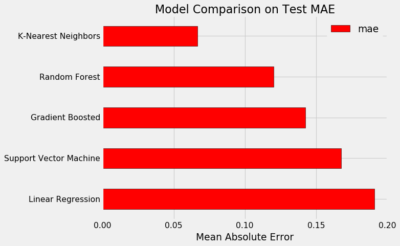
11. Hyperparameter Tuning
Clearly, KNeighborsRegressor gives us the best MAE. Now we can tweak it’s hyperparameters to gain even more accuracy. This task becomes really easy because of RandomizedSearchCV provided by scikit-learn.
# Loss function to be optimized
n_neighbors = [2, 5, 8, 11, 14]

weights = ['uniform', 'distance']

algorithm  = ['ball_tree', 'kd_tree', 'brute']

leaf_size = [10,20,30,40,50,60]

p = [1,2]

# Number of trees used in the boosting process
n_estimators = [100, 500, 900, 1100, 1500]

# Maximum depth of each tree
max_depth = [2, 3, 5, 10, 15]

# Minimum number of samples per leaf
min_samples_leaf = [1, 2, 4, 6, 8]

# Minimum number of samples to split a node
min_samples_split = [2, 4, 6, 10]

# Maximum number of features to consider for making splits
max_features = ['auto', 'sqrt', 'log2', None]

# Define the grid of hyperparameters to search
hyperparameter_grid = {'n_neighbors': n_neighbors,
                       'weights': weights,
                       'algorithm': algorithm,
                       'leaf_size': leaf_size,
                       'p': p}

# Create the model to use for hyperparameter tuning
model = KNeighborsRegressor()

random_cv = RandomizedSearchCV(estimator=model,
                               param_distributions=hyperparameter_grid,
                               cv=4, n_iter=25,
                               scoring = 'neg_mean_absolute_error',
                               n_jobs = -1, verbose = 1,
                               return_train_score = True)
random_cv.fit(X, y)
We can view the results of this step in the following way:
random_results = pd.DataFrame(random_cv.cv_results_).sort_values('mean_test_score', ascending = False)

random_results.head(5)
| mean_fit_time | std_fit_time | mean_score_time | std_score_time | param_weights | param_p | param_n_neighbors | param_leaf_size | param_algorithm | params | split0_test_score | split1_test_score | split2_test_score | split3_test_score | mean_test_score | std_test_score | rank_test_score | split0_train_score | split1_train_score | split2_train_score | split3_train_score | mean_train_score | std_train_score | |
| 1 | 0.00000 | 0.000000 | 0.05225 | 0.022487 | uniform | 1 | 2 | 10 | brute | {‘weights’: ‘uniform’, ‘p’: 1, ‘n_neighbors’: … | -0.032258 | -0.032258 | -0.048387 | -0.032258 | -0.036290 | 0.006984 | 1 | -0.026882 | -0.010753 | -0.016129 | -0.021505 | -0.018817 | 0.006011 |
| 15 | 0.00025 | 0.000433 | 0.00050 | 0.000500 | distance | 1 | 2 | 20 | kd_tree | {‘weights’: ‘distance’, ‘p’: 1, ‘n_neighbors’:… | -0.032333 | -0.034299 | -0.046358 | -0.033374 | -0.036591 | 0.005682 | 2 | -0.000000 | -0.000000 | -0.000000 | -0.000000 | 0.000000 | 0.000000 |
| 23 | 0.00025 | 0.000433 | 0.00050 | 0.000500 | uniform | 2 | 2 | 40 | ball_tree | {‘weights’: ‘uniform’, ‘p’: 2, ‘n_neighbors’: … | -0.064516 | -0.048387 | -0.048387 | -0.048387 | -0.052419 | 0.006984 | 3 | -0.032258 | -0.032258 | -0.021505 | -0.026882 | -0.028226 | 0.004458 |
| 18 | 0.00025 | 0.000433 | 0.00025 | 0.000433 | distance | 2 | 2 | 40 | kd_tree | {‘weights’: ‘distance’, ‘p’: 2, ‘n_neighbors’:… | -0.065504 | -0.051098 | -0.047090 | -0.048416 | -0.053027 | 0.007347 | 4 | -0.000000 | -0.000000 | -0.000000 | -0.000000 | 0.000000 | 0.000000 |
| 6 | 0.00025 | 0.000433 | 0.00075 | 0.000433 | distance | 2 | 2 | 60 | ball_tree | {‘weights’: ‘distance’, ‘p’: 2, ‘n_neighbors’:… | -0.065504 | -0.051098 | -0.047090 | -0.048416 | -0.053027 | 0.007347 | 4 | -0.000000 | -0.000000 | -0.000000 | -0.000000 | 0.000000 | 0.000000 |
Here we can see the best estimator:
random_cv.best_estimator_
Let’s see if leaf size plays an important role here by using GridSearchCV:
# Create a range of leaves to evaluate
leaves_grid = {'leaf_size': [3, 5, 7, 9, 10, 11, 13, 15, 17]}

model = KNeighborsRegressor(algorithm='brute', leaf_size=10, metric='minkowski',
          metric_params=None, n_jobs=1, n_neighbors=2, p=1,
          weights='uniform')

# Grid Search Object using the trees range and our model
grid_search = GridSearchCV(estimator = model, param_grid=leaves_grid, cv = 4,
                           scoring = 'neg_mean_absolute_error', verbose = 1,
                           n_jobs = -1, return_train_score = True)
# Fit the grid search
grid_search.fit(X, y)
We can see the results in a similar manner:
# Get the results into a dataframe
results = pd.DataFrame(grid_search.cv_results_)
results.head(5)
| mean_fit_time | std_fit_time | mean_score_time | std_score_time | param_leaf_size | params | split0_test_score | split1_test_score | split2_test_score | split3_test_score | mean_test_score | std_test_score | rank_test_score | split0_train_score | split1_train_score | split2_train_score | split3_train_score | mean_train_score | std_train_score | |
| 0 | 0.00050 | 0.000500 | 0.00025 | 0.000433 | 3 | {‘leaf_size’: 3} | -0.032258 | -0.032258 | -0.048387 | -0.032258 | -0.03629 | 0.006984 | 1 | -0.026882 | -0.010753 | -0.016129 | -0.021505 | -0.018817 | 0.006011 |
| 1 | 0.00025 | 0.000433 | 0.00025 | 0.000433 | 5 | {‘leaf_size’: 5} | -0.032258 | -0.032258 | -0.048387 | -0.032258 | -0.03629 | 0.006984 | 1 | -0.026882 | -0.010753 | -0.016129 | -0.021505 | -0.018817 | 0.006011 |
| 2 | 0.00025 | 0.000433 | 0.00050 | 0.000500 | 7 | {‘leaf_size’: 7} | -0.032258 | -0.032258 | -0.048387 | -0.032258 | -0.03629 | 0.006984 | 1 | -0.026882 | -0.010753 | -0.016129 | -0.021505 | -0.018817 | 0.006011 |
| 3 | 0.00000 | 0.000000 | 0.00025 | 0.000433 | 9 | {‘leaf_size’: 9} | -0.032258 | -0.032258 | -0.048387 | -0.032258 | -0.03629 | 0.006984 | 1 | -0.026882 | -0.010753 | -0.016129 | -0.021505 | -0.018817 | 0.006011 |
| 4 | 0.00000 | 0.000000 | 0.00025 | 0.000433 | 10 | {‘leaf_size’: 10} | -0.032258 | -0.032258 | -0.048387 | -0.032258 | -0.03629 | 0.006984 | 1 | -0.026882 | -0.010753 | -0.016129 | -0.021505 | -0.018817 | 0.006011 |
Plot our findings:
# Plot the training and testing error vs number of trees
figsize(8, 8)
plt.style.use('fivethirtyeight')
plt.plot(results['param_leaf_size'], -1 * results['mean_test_score'], label = 'Testing Error')
plt.plot(results['param_leaf_size'], -1 * results['mean_train_score'], label = 'Training Error')
plt.xlabel('Leaf Size'); plt.ylabel('Mean Abosolute Error'); plt.legend();
plt.title('Performance vs Number of Trees');
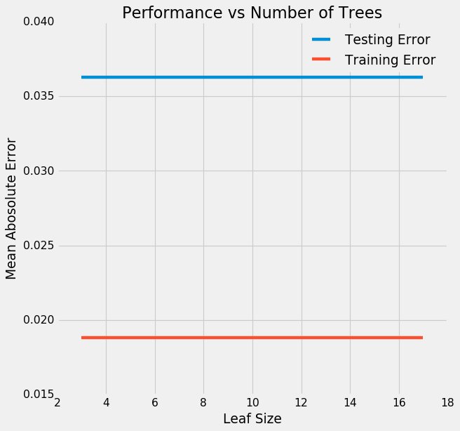
Well, it does not!
12. Present your gains
It is important that we present how much impact our performance tuning made. So, we’ll take our default model & our best model and contrast their accuracy along with performance.
# Default model
default_model = KNeighborsRegressor(5)

# Select the best model
final_model = grid_search.best_estimator_

final_model
%%timeit -n 1 -r 5
default_model.fit(X, y)
%%timeit -n 1 -r 5
final_model.fit(X, y)
We are in luck, our final model is faster than our default model. Let’s check performance:
default_pred = default_model.predict(X_test)
final_pred = final_model.predict(X_test)

print('Default model performance on the test set: MAE = %0.4f.' % mae(y_test, default_pred))
print('Final model performance on the test set:   MAE = %0.4f.' % mae(y_test, final_pred))
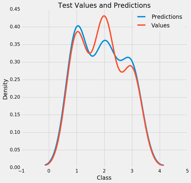
Aaaand it is more accurate ! If we plot this:
figsize(8, 8)

# Density plot of the final predictions and the test values
sns.kdeplot(final_pred, label = 'Predictions')
sns.kdeplot(y_test, label = 'Values')

# Label the plot
plt.xlabel('Class'); plt.ylabel('Density');
plt.title('Test Values and Predictions');
13. Plotting residuals
figsize = (6, 6)

# Calculate the residuals
residuals = final_pred - y_test

# Plot the residuals in a histogram
plt.hist(residuals, color = 'red', bins = 20,
         edgecolor = 'black')
plt.xlabel('Error'); plt.ylabel('Count')
plt.title('Distribution of Residuals');
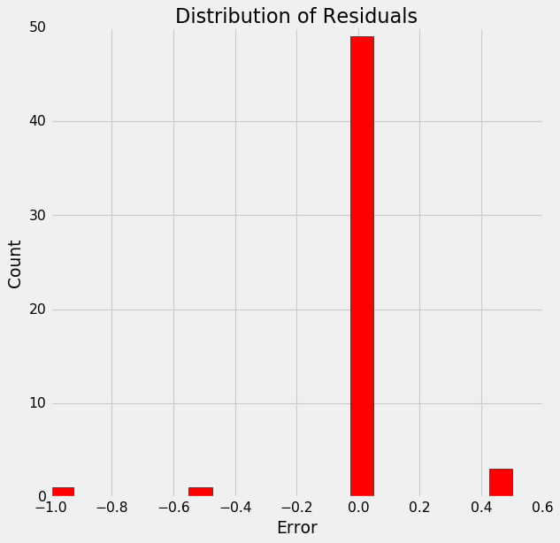
This somewhat of a normal distribution and supports our model’s accuracy.
Summary
We learned how to compare models, tuning the best one using it’s hyperparameters and visualizing results in an effective way. Note that the values I got might differ in your case because of the inherent randomness in every algorithm. Also, here we only discussed GridSearch on a single parameter, but you can do it on multiple parameters to increase your model’s accuracy.