My first dig on sentiment analysis using IMDb reviews

The past fifteen years have seen extensive investments in business infrastructure, which have improved the ability to collect data throughout the enterprise. Virtually every aspect of business is now open to data collection and often even instrumented for data collection: operations, manufacturing, supply-chain management, customer behavior, marketing campaign performance, workflow procedures, and so on. This broad availability of data has led to increasing interest in methods for extracting useful information and knowledge from data—the realm of data science. This realm is huge. To understand the whole picture, we have to go through the individual building blocks; specific algorithms being used for specific tasks. Let’s consider the case of retail industry. Some of the use cases exploiting Data Science tools are:

• Recommendation engines: compute a similarity index in the customers’ preferences and offer the goods or services accordingly.
• Fraud detection: continuous monitoring of the activity and ensure the detection of the fraudulent activity.
• Customer sentiment analysis: analysts can perform the brand-customer sentiment analysis by data received from social networks and online services feedbacks.

There are hundreds of other examples. Consider the fellows at Gradient, who showcased at CES 2019, a technology allows companies to offer an extra level of security in online processes.

Let us take a small piece of the pie and understand it on a deeper level: consider a case study on Sentiment Analysis.

Data

For this analysis we’ll be using a dataset of 50,000 movie reviews taken from IMDb. The data was compiled by Andrew Maas and can be found here: IMDb Reviews. The data is split evenly with 25k reviews intended for training and 25k for testing your classifier. Moreover, each set has 12.5k positive and 12.5k negative reviews. IMDb lets us rate movies on a scale from 1 to 10. To label these reviews the curator of the data labeled anything with ≤ 4 stars as negative and anything with ≥ 7 stars as positive. Reviews with 5 or 6 stars were left out.

First import the essentials:

from sklearn.feature_extraction.text import TfidfVectorizer
from sklearn.metrics import accuracy_score
import numpy as np
import pandas as pd
import os
import re

Then, read the training and validation files:

reviews_train = []
for line in open('C:/Users/SOUMYA/Downloads/movie_data.tar/movie_data/movie_data/full_train.txt', encoding="utf8"): 
    reviews_train.append(line.strip())
reviews_test = []
for line in open('C:/Users/SOUMYA/Downloads/movie_data.tar/movie_data/movie_data/full_test.txt', encoding="utf8"):
    reviews_test.append(line.strip())
reviews_train[5]

Ok. So we have successfully imported the required files. Now, as you can imagine, special characters (like ‘,’ ‘-‘ ‘,’ ‘/’ etc) and numbers are not essential for a sentiment analysis. Hence, we write a function to eliminate these characters using regular expression (re) :

REPLACE_NO_SPACE = re.compile("(\.)|(\;)|(\:)|(\!)|(\')|(\?)|(\,)|(\")|(\()|(\))|(\[)|(\])|(\d+)")
REPLACE_WITH_SPACE = re.compile("(<br\s*/><br\s*/>)|(\-)|(\/)")
def preprocess_reviews(reviews):
    reviews = [REPLACE_NO_SPACE.sub("", line.lower()) for line in reviews]
    reviews = [REPLACE_WITH_SPACE.sub(" ", line) for line in reviews] 
    return reviews

reviews_train_clean = preprocess_reviews(reviews_train)
reviews_test_clean = preprocess_reviews(reviews_test)
reviews_train_clean[5]

Food for thought: Why did we use two variables REPLACE_NO_SPACE and REPLACE_WITH_SPACE?

Vectorization

In order for this data to make sense to our machine learning algorithm we’ll need to convert each review to a numeric representation, which we call vectorization. The simplest way to implement this is by one hot encoding:

from sklearn.feature_extraction.text import CountVectorizer
cv = CountVectorizer(binary=True)
cv.fit(reviews_train_clean)
X = cv.transform(reviews_train_clean)
X_test = cv.transform(reviews_test_clean)

Building the Classifier

Now, we build the classifier. We can choose from numerous algorithms but I’m going to go with Logistic Regression as our baseline model because they’re easy to interpret, fast and its performance on sparse datasets like ours. Note: The targets/labels we use will be the same for training and testing because both datasets are structured the same, where the first 12.5k are positive and the last 12.5k are negative. Also I should point out that there are several hyper-parameters associated with all regression algorithms but I’m only going to concentrate on c (which adjusts regularization) to keep things simple.

from sklearn.linear_model import LogisticRegression
from sklearn.metrics import accuracy_score
from sklearn.model_selection import train_test_split

target = [1 if i < 12500 else 0 for i in range(25000)]
X_train, X_val, y_train, y_val = train_test_split(
    X, target, train_size = 0.75
)
for c in [0.01, 0.05, 0.25, 0.5, 1]:
    lr = LogisticRegression(C=c)
    lr.fit(X_train, y_train)
    print ("Accuracy for C=%s: %s" 
           % (c, accuracy_score(y_val, lr.predict(X_val))))

We get highest accuracy with c=0.05. If we were to stop here, we would select our final model with c=0.05.

Removing Stop Words

To go one step further, we will try and remove any stop words from our input text. Stop words are the very common words like ‘if’, ‘but’, ‘we’, ‘he’, ‘she’, and ‘they’. We can usually remove these words without changing the semantics of a text and doing so often (but not always) improves the performance of a model. Removing these stop words becomes a lot more useful when we start using longer word sequences as model features (see n-grams below). This can be done by a couple of ways:

1. using stop words from nltk and making an udf to remove words
2. using manual stop words and making an udf to remove words (we will see this in our final model)
3. using countVectorizer

from nltk.corpus import stopwords

english_stop_words = stopwords.words('english')
def remove_stop_words(corpus):
    removed_stop_words = []
    for review in corpus:
        removed_stop_words.append(
            ' '.join([word for word in review.split() 
                      if word not in english_stop_words])
        )
    return removed_stop_words

no_stop_words = remove_stop_words(reviews_train_clean)

Before:

After:

Normalization

Next up is text Normalization in which we try to convert all of the different forms of a given word into one. Most common 2 methods are Stemming and Lemmatization. The goal of both stemming and lemmatization is to reduce inflectional forms and sometimes derivationally related forms of a word to a common base form. However, the two words differ in their flavor. Stemming usually refers to a crude heuristic process that chops off the ends of words in the hope of achieving this goal correctly most of the time, and often includes the removal of derivational affixes. Lemmatization usually refers to doing things properly with the use of a vocabulary and morphological analysis of words, normally aiming to remove inflectional endings only and to return the base or dictionary form of a word, which is known as the lemma . For our tutorial here, I’m going with Lemmatization.

def get_lemmatized_text(corpus):
    from nltk.stem import WordNetLemmatizer
    lemmatizer = WordNetLemmatizer()
    return [' '.join([lemmatizer.lemmatize(word) for word in review.split()]) for review in corpus]
lemmatized_reviews_train = get_lemmatized_text(reviews_train_clean)
lemmatized_reviews_test = get_lemmatized_text(reviews_test_clean)

print('before lemmatization\n------------------------\n',reviews_train_clean[5],'\n\nafter lemmatization\n------------------------\n',lemmatized_reviews_train[5])

n-grams

Consider n-grams. Up until now, we used only single word features in our model, which we call 1-grams or unigrams. We can potentially add more predictive power to our model by adding two or three word sequences (bigrams or trigrams) as well. For example, if a review had the three word sequence “didn’t love movie” we would only consider these words individually with a unigram-only model and probably not capture that this is actually a negative sentiment because the word ‘love’ by itself is going to be highly correlated with a positive review.

cv = CountVectorizer(binary=True, ngram_range=(1, 2))
cv.fit(lemmatized_reviews_train)
X = cv.transform(lemmatized_reviews_train)
X_test = cv.transform(lemmatized_reviews_test)

X_train, X_val, y_train, y_val = train_test_split(
    X, target, train_size = 0.75
)

for c in [0.01, 0.05,0.06,0.07,0.08, 0.25, 0.5, 1]:
    lr = LogisticRegression(C=c)
    lr.fit(X_train, y_train)
    print ("Accuracy for C=%s: %s" 
           % (c, accuracy_score(y_val, lr.predict(X_val))))

Note: There’s technically no limit on the size that n can be for your model, but there are several things to consider. First, increasing the number of grams will not necessarily give you better performance. Second, the size of your matrix grows exponentially as you increment n, so if you have a large corpus that is comprised of large documents your model may take a very long time to train.

Algorithms

As I said earlier, there are a variety of algorithms to choose from. So far we’ve chosen to represent each review as a very sparse vector (lots of zeros!) with a slot for every unique n-gram in the corpus (minus n-grams that appear too often or not often enough). Linear classifiers typically perform better than other algorithms on data that is represented in this way. So far we’ve chosen to represent each review as a very sparse vector (lots of zeros!) with a slot for every unique n-gram in the corpus (minus n-grams that appear too often or not often enough). Linear classifiers typically perform better than other algorithms on data that is represented in this way. Another algorithm that can produce great results with a quick training time are Support Vector Machines with a linear kernel. Here is an example:

from sklearn.svm import LinearSVC
ngram_vectorizer = CountVectorizer(binary=True, ngram_range=(1, 2))
ngram_vectorizer.fit(reviews_train_clean)
X = ngram_vectorizer.transform(reviews_train_clean)
X_test = ngram_vectorizer.transform(reviews_test_clean)

X_train, X_val, y_train, y_val = train_test_split(
    X, target, train_size = 0.75
)

for c in [0.01, 0.05, 0.25, 0.5, 1]:
    
    svm = LinearSVC(C=c)
    svm.fit(X_train, y_train)
    print ("Accuracy for C=%s: %s" 
           % (c, accuracy_score(y_val, svm.predict(X_val))))

Final Model

Finally, let’s make our final model:

from sklearn.feature_extraction.text import CountVectorizer
from sklearn.model_selection import train_test_split
from sklearn.metrics import accuracy_score
from sklearn.svm import LinearSVC


stop_words = ['in', 'of', 'at', 'a', 'the']
ngram_vectorizer = CountVectorizer(binary=True, ngram_range=(1, 3), stop_words=stop_words)
ngram_vectorizer.fit(reviews_train_clean)
X = ngram_vectorizer.transform(reviews_train_clean)
X_test = ngram_vectorizer.transform(reviews_test_clean)

X_train, X_val, y_train, y_val = train_test_split(
    X, target, train_size = 0.75
)

for c in [0.001, 0.005, 0.01, 0.05, 0.1]:
    
    svm = LinearSVC(C=c)
    svm.fit(X_train, y_train)
    print ("Accuracy for C=%s: %s" 
           % (c, accuracy_score(y_val, svm.predict(X_val))))

final = LinearSVC(C=0.1)
final.fit(X, target)
print ("Final Accuracy: %s" 
       % accuracy_score(target, final.predict(X_test)))

Pretty close to 90!

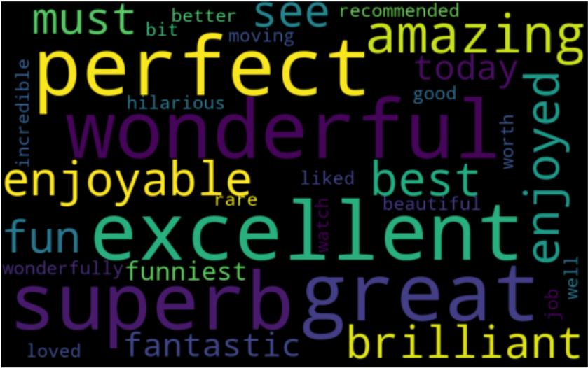
Visualization

Visualizing the most defining words/phrases is a good way to check your model’s sanity. One way of doing this is by using WordCloud:

feature_to_coef = {
    word: coef for word, coef in zip(
        ngram_vectorizer.get_feature_names(), final.coef_[0]
    )
}

positive_words=[]

for best_positive in sorted(
    feature_to_coef.items(), 
    key=lambda x: x[1], 
    reverse=True)[:30]:
    positive_words.append(best_positive[0])

best_positive_words = ' '.join(positive_words)
from wordcloud import WordCloud
import matplotlib.pyplot as plt
wordcloud = WordCloud(width=800, height=500, random_state=21, max_font_size=110).generate(best_positive_words)

plt.figure(figsize=(10, 7))
plt.imshow(wordcloud, interpolation="bilinear")
plt.axis('off')
plt.show()

negative_words=[]
for best_negative in sorted(
    feature_to_coef.items(), 
    key=lambda x: x[1], 
    reverse=False)[:30]:
    negative_words.append(best_negative[0])
best_neg_words = ' '.join(negative_words)
wordcloud = WordCloud(width=800, height=500, random_state=21, max_font_size=110).generate(best_neg_words)

plt.figure(figsize=(10, 7))
plt.imshow(wordcloud, interpolation="bilinear")
plt.axis('off')
plt.show()

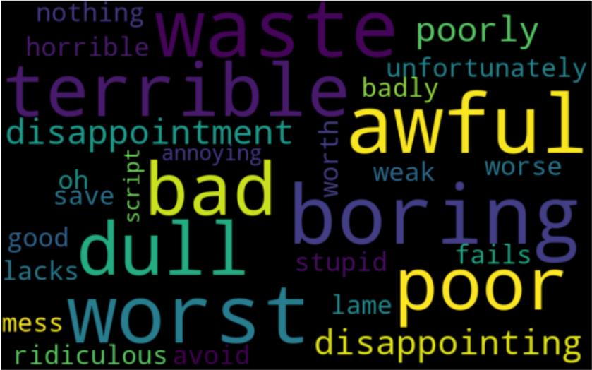
Clearly these results make sense.

Summary

We’ve gone over several options for transforming text that can improve the accuracy of an NLP model. Which combination of these techniques will yield the best results will depend on the task, data representation, and algorithms you choose. It’s always a good idea to try out many different combinations to see what works.